Welcome to Jupyter Notebook Tutorial by AIMLC, IITD

--- prepared by Nirjhar Das.

In this notebook, we will get familiar with the Jupyter environment and also explore the powerful Python libraries:

Pandas
NumPy
Matplotlib

If you are more the video-watching kind rather than the reading kind, or even if you would just like to have someone guide you through everything in this post, we have a great set of tutorial videos. Watch them on YouTube or find them below. Follow along with the videos and come back for the code whenever you want to;) Stay tuned for Part 3!

Package installation and import

If you have installed Anaconda then these packages are already installed, so you can proceed to the next block of codes.

Otherwise, if you have only Python 3.x installed in your computer, then you have to install these packages separately. At your terminal/cmd run the following commands

pip3 install numpy pandas matplotlib

[ Note: You need internet connectivity to download and install these packages using the pip3 command ]

Once the packages are installed, proceed to the next block of codes given below.

#import all the necessary packages
import numpy as np
import pandas as pd
import matplotlib.pyplot as plt
%matplotlib inline

Data loading with Pandas

Pandas is the perfect package for handling tabular data. It has awesome methods to manipulate and perform calculations on the data. The data is read as an object called DATAFRAME in Pandas. The dataframe holds the whole table of data and supports functions to work in data.

Find out more in the official documentation.

Let's take a look into some examples. If you have the data file "StudentPerformance.csv" in the same folder as this notebook, then you are good to go. Else, you can download it here in the .zip format. Extract the file from the archive and place it in the same directory as this notebook.

#Now that the packages are installed, we can load the data into the program
df = pd.read_csv('StudentsPerformance.csv')
print('Number of entries =', len(df))
df.head(10)

Number of entries = 1000

	gender	race/ethnicity	parental level of education	lunch	test preparation course	math score	reading score	writing score
0	female	group B	bachelor's degree	standard	none	72	72	74
1	female	group C	some college	standard	completed	69	90	88
2	female	group B	master's degree	standard	none	90	95	93
3	male	group A	associate's degree	free/reduced	none	47	57	44
4	male	group C	some college	standard	none	76	78	75
5	female	group B	associate's degree	standard	none	71	83	78
6	female	group B	some college	standard	completed	88	95	92
7	male	group B	some college	free/reduced	none	40	43	39
8	male	group D	high school	free/reduced	completed	64	64	67
9	female	group B	high school	free/reduced	none	38	60	50

You can see that there are 1000 rows in table. Each row correspond to an observation (student) and the columns are the features pertaining to the observations. Typical Machine Learning requires you to extract features from a raw data file (say, some website, or some software). In this case, the data has already been collected and stored in a .csv file.

Once the data is collected, the pipeline involves Exploratory Data Analysis (EDA), where the engineer looks into the data and tries to figure out statistics and correlations. Let's do some basic EDA now.

#Let's get an idea of the different types of data values present in each column (except the last three)
col_dict = {}
for col in df.columns[:-3]:
    col_dict[col] = list(df[col].unique())
print(col_dict)

{'gender': ['female', 'male'], 'race/ethnicity': ['group B', 'group C', 'group A', 'group D', 'group E'], 'parental level of education': ["bachelor's degree", 'some college', "master's degree", "associate's degree", 'high school', 'some high school'], 'lunch': ['standard', 'free/reduced'], 'test preparation course': ['none', 'completed']}

for key in col_dict:
    print('Distribution of values for', key)
    print(df[key].value_counts(), end='\n\n')

Distribution of values for gender
female    518
male      482
Name: gender, dtype: int64

Distribution of values for race/ethnicity
group C    319
group D    262
group B    190
group E    140
group A     89
Name: race/ethnicity, dtype: int64

Distribution of values for parental level of education
some college          226
associate's degree    222
high school           196
some high school      179
bachelor's degree     118
master's degree        59
Name: parental level of education, dtype: int64

Distribution of values for lunch
standard        645
free/reduced    355
Name: lunch, dtype: int64

Distribution of values for test preparation course
none         642
completed    358
Name: test preparation course, dtype: int64

Now that we have an idea of the categorical data values, let us look at some statistics related to the numerical data values.

df.describe()

	math score	reading score	writing score
count	1000.00000	1000.000000	1000.000000
mean	66.08900	69.169000	68.054000
std	15.16308	14.600192	15.195657
min	0.00000	17.000000	10.000000
25%	57.00000	59.000000	57.750000
50%	66.00000	70.000000	69.000000
75%	77.00000	79.000000	79.000000
max	100.00000	100.000000	100.000000

Digression

Here, I would like to point out that in most cases, numerical data is standardized/normalized before further processing. This is because most of Machine Learning algortihms give better result with Standard data. This step is particularly important when data values belong to different scales (for e.g. height vs. weight which have different units). Also, in Neural Networks, things (I mean, parameter values) may explode if data is not normalized/standardized.

How to standardize data?
A normal distribution is one in which mean ( $\mu$ ) = 0.0 and standard deviation ( $\sigma$ ) = 1.0
So, for a set of observations of random variable x do
$x^\prime = \frac{x - \mu}{\sigma}$

Python Code for standardization

s, sq_s, n = 0.0, 0.0, 0.0
for x in observed_dataset:
    s = s + x
    sq_s = sq_s + (x*x)
    n = n + 1.0

mean = s/n
sq_mean = sq_s/n
std = math.sqrt(sq_mean - (mean*mean))

new_dataset = []
for x in observed_dataset:
    x_new = (x - mean)/std
    new_dataset.append(x_new)

How to normalize data?
A normalized data is such that $x \in [0, 1]$
So for a set of observations of $x$ do:
$x^\prime = \frac{x - x_{min}}{x_{max} - x_{min}}$

Python code for normalization

min_x = min(observed_dataset)
max_x = max(observed_dataset)
new_dataset = [(x - min_x)/(max_x - min_x) for x in observed_dataset]

But!

We don't do that here

Let's unlock the power of NumPy.

#Let's take an example
math_score = np.array(df['math score'])
std_math_score = (math_score - np.mean(math_score))/np.std(math_score) #That's it! It's standardized!

#Create a column in dataframe and add the standardized scores
df['standardized math score'] = std_math_score
#To cross-check:
df['standardized math score'].describe()

count    1.000000e+03
mean     8.704149e-17
std      1.000500e+00
min     -4.360728e+00
25%     -5.997164e-01
50%     -5.872457e-03
75%      7.199368e-01
max      2.237538e+00
Name: standardized math score, dtype: float64

Note: mean $\sim 10^{-17}$ which is very close to $0.0$ . Similarly, std $\approx 1.0$ . The error remains due to some internal computation.

#Normalizing data
norm_math_score = (math_score - np.min(math_score))/(np.max(math_score) - np.min(math_score))
df['normalized math score'] = norm_math_score
df['normalized math score'].describe()

count    1000.000000
mean        0.660890
std         0.151631
min         0.000000
25%         0.570000
50%         0.660000
75%         0.770000
max         1.000000
Name: normalized math score, dtype: float64

Note: min $= 0.0$ , max $= 1.0$ . Thus, every value $\in [0, 1]$

Power of NumPy

NumPy is the Linear Algebra library of Python. It lets you manipulate matrices and perform wide range of matrix operations. Find out more about this amazing library from the official documentation.

#Let's look at a few examples
A = np.random.rand(5, 5) #Define a matrix of size 5x5 filled with random values
B = np.random.normal(0.0, 1.0, size=(5, 3)) #Define a matrix of size 5x3 filled with random values from a Normal Distribution
C = np.zeros((3, 2)) #A matrix filled with zeros
I = np.eye(5) #An identity matrix of order 5
v = np.random.rand(5) #A vector of size 5x1
u = np.random.uniform(low=-1.0, high=1.0, size=5) #A vector of size 5x1 with uniform sampling between low and high

print('A =')
print(A, end='\n\n')
print('B =')
print(B, end='\n\n')
print('C =')
print(C, end='\n\n')
print('I =')
print(I, end='\n\n')
print('v =')
print(v, end='\n\n')
print('u =')
print(u, end='\n\n')

A =
[[0.62783835 0.28592923 0.75280145 0.1894534  0.64469173]
 [0.00430482 0.37667124 0.50444169 0.57647561 0.29948052]
 [0.47515683 0.17642003 0.93427809 0.95568321 0.22061894]
 [0.47081525 0.26964797 0.67040647 0.83297107 0.74845429]
 [0.38895193 0.90094653 0.28856394 0.70228856 0.34101627]]

B =
[[ 0.15843576  2.45183925 -0.33868413]
 [ 0.06052418  0.44717844  0.92390245]
 [ 0.55750733  0.43016366  0.0322283 ]
 [-0.8962773  -0.55301244 -0.98375332]
 [ 2.40044793 -0.03392459 -1.3648234 ]]

C =
[[0. 0.]
 [0. 0.]
 [0. 0.]]

I =
[[1. 0. 0. 0. 0.]
 [0. 1. 0. 0. 0.]
 [0. 0. 1. 0. 0.]
 [0. 0. 0. 1. 0.]
 [0. 0. 0. 0. 1.]]

v =
[0.27208837 0.4580093  0.56672388 0.13323657 0.29509171]

u =
[-0.438004    0.24642209  0.14904029  0.18685347  0.43908568]

#Element-wise squaring a matrix
print('A**2 =\n', A**2, end='\n\n')

#Matrix squaring
print('A^2 =\n', np.matmul(A, A), end='\n\n')

#Matrix multiplication
print('A x B =\n', A@B)
print('Shape =', (A@B).shape, end='\n\n') #Note: Shape should be (5, 3)

#Matrix-vector multiplication
print('I.v =\n', np.dot(I, v), end='\n\n')

#Transpose
print('C\' =\n', C.T)
print(C.T.shape, end='\n\n')

#Dot product
print('u\'.v =\n', np.dot(u, v))

#Addition/Substraction is just simple +/- but size should match

A**2 =
 [[3.94180989e-01 8.17555244e-02 5.66710027e-01 3.58925925e-02
  4.15627433e-01]
 [1.85315078e-05 1.41881221e-01 2.54461417e-01 3.32324129e-01
  8.96885802e-02]
 [2.25774010e-01 3.11240278e-02 8.72875547e-01 9.13330401e-01
  4.86727153e-02]
 [2.21666998e-01 7.27100271e-02 4.49444840e-01 6.93840796e-01
  5.60183821e-01]
 [1.51283605e-01 8.11704647e-01 8.32691466e-02 4.93209228e-01
  1.16292094e-01]]

A^2 =
 [[1.09306226 1.05194641 1.63324372 1.61378589 1.01812226]
 [0.63191018 0.65736712 1.13743043 1.39055304 0.76046374]
 [1.27877014 0.82360285 2.0239268  2.03559043 1.35580332]
 [1.29859309 1.25338786 1.89120427 2.10481092 1.41086523]
 [0.84847758 0.99808994 1.58610133 1.69331556 1.22615568]]

A x B =
 [[ 1.91421616  1.86440692 -0.99047243]
 [ 0.50691508  0.06702854 -0.61304101]
 [ 0.2798535   1.10980276 -1.2090854 ]
 [ 1.51472321  1.0772942  -1.72966915]
 [ 0.46617595  1.08071805 -0.44635091]]
Shape = (5, 3)

I.v =
 [0.27208837 0.4580093  0.56672388 0.13323657 0.29509171]

C' =
 [[0. 0. 0.]
 [0. 0. 0.]]
(2, 3)

u'.v =
 0.2326187640932555

Finally, let's discuss about Matplotlib

Matplotlib is the Python library for plotting graphs and figures. Here we will look at a few examples.

Find out more about this library from the official documentation.

#Plotting a histogram
plt.figure(figsize=(7, 5))
plt.xticks(np.arange(0.0, 105.0, 5.0))
plt.xlabel('Reading Score')
plt.ylabel('No. of students')
_, _, _ = plt.hist(x=df['reading score'], bins=20, range=(0.0, 100.0), edgecolor='black')
plt.show()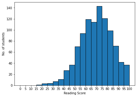

png

#Scatter Plot to observe the correlation
plt.figure(figsize=(10, 10))
plt.grid(True, linewidth=0.5, color='gray', linestyle='-')
plt.xlabel('Reading Score')
plt.ylabel('Writing Score')
plt.xticks(np.arange(0.0, 105.0, 5.0))
plt.yticks(np.arange(0.0, 105.0, 5.0))
plt.scatter(x=df['reading score'], y=df['writing score'], s=10.0, color='orange', marker='+')
plt.show()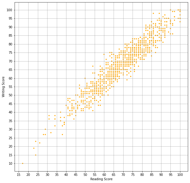

png

Conclusion

In this tutorial, we learnt the basics of Pandas, NumPy and Matplotlib. There are many more awesome things you can do with these packages. As you set out to explore the world of Data Science and Machine Learning, you will get to know more about these libraries and several others. There are plenty of resources available in the Internet as well as there are good books on the topic. Moreover, since you are a part of AIMLC, we will make sure that you have the right resources and learning environment.